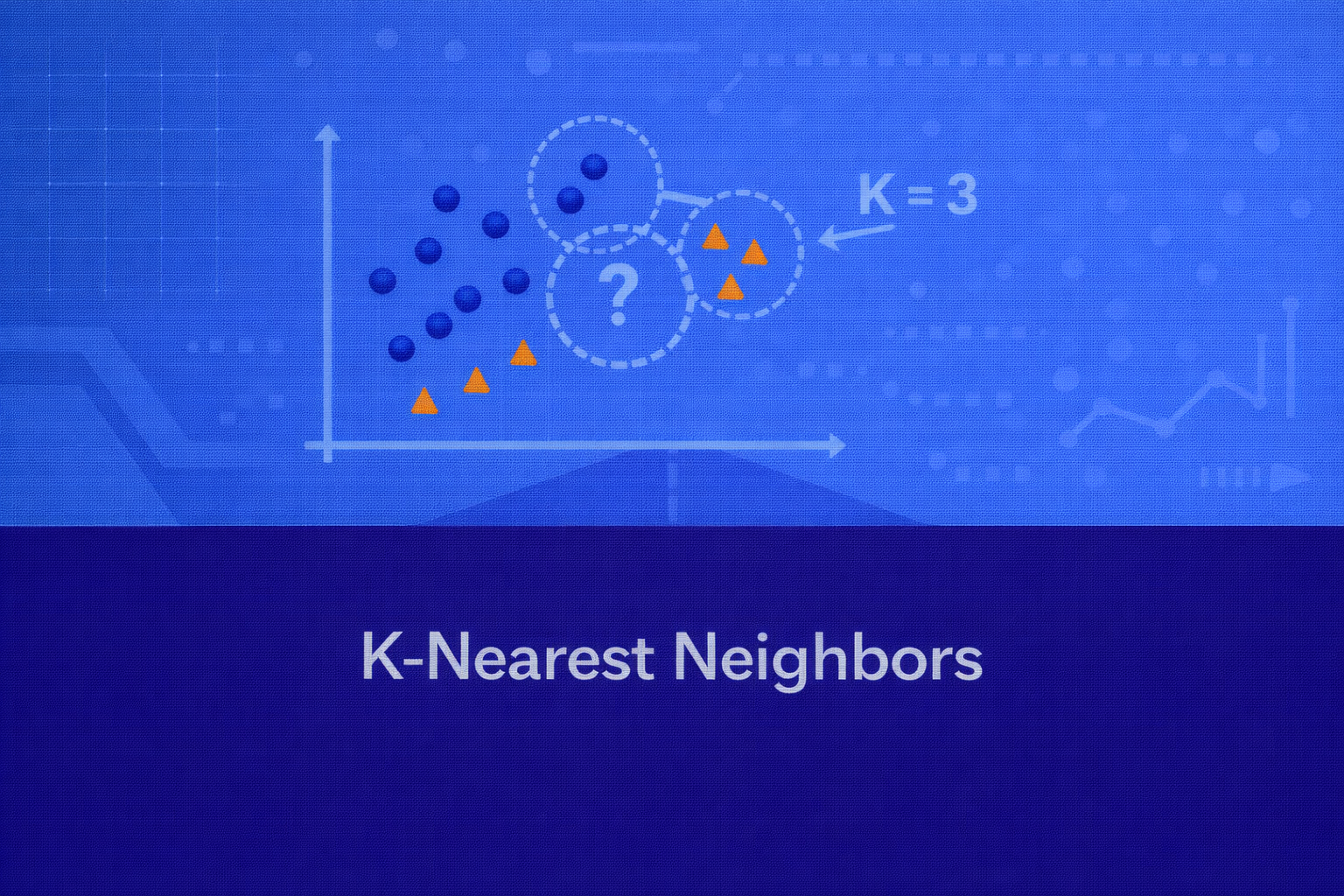
K-Nearest Neighbors (KNN) – Dev Nexus Hub by Uma Mahesh

K-Nearest Neighbors (KNN) is one of the most intuitive non-parametric supervised learning algorithms. It is used for both classification and regression, and it operates on a simple idea: similar observations tend to have similar outputs. Unlike models that explicitly learn a compact parametric function during training, KNN postpones most of the computation until prediction time. Because of this, it is often described as a lazy learner or instance-based learner.

Abstract

This whitepaper presents a detailed technical treatment of K-Nearest Neighbors for both classification and regression. It covers the mathematical intuition, training and inference behavior, distance metrics, feature scaling requirements, curse of dimensionality, bias-variance trade-offs, model selection, computational complexity, interpretability, advantages, limitations, and practical deployment considerations. Formulas are embedded inline in HTML-friendly format so they can be pasted directly into WordPress or similar editors.

1. Introduction

KNN belongs to the family of supervised learning methods in which predictions are based on labeled examples. Given a query point, the algorithm looks for the k closest training examples according to a chosen distance function and then uses those neighbors to infer the target. In classification, the output is generally the majority class among the neighbors. In regression, the output is usually the average or weighted average of their target values.

If the training dataset is D = {(x_i, y_i)}_i=1ⁿ, where x_i ∈ ℝ^p is a feature vector and y_i is the label or response, then for a new query point x, KNN first computes distances d(x, x_i) to all training examples, sorts them, and selects the nearest k.

2. Core Intuition

The core assumption behind KNN is local smoothness: if two points are close in feature space, their outputs are expected to be similar. In a geometric sense, KNN constructs a local neighborhood around the query point and lets the training samples in that neighborhood vote or average. Unlike linear models such as ŷ = Xβ, KNN does not assume a global linear relationship. Unlike tree-based models, it does not partition the feature space using learned rules. Instead, its prediction is entirely driven by proximity.

3. KNN for Classification

For binary or multiclass classification, let N_k(x) denote the set of indices corresponding to the k nearest neighbors of query point x. The basic unweighted KNN classifier predicts the class ŷ as the majority vote:

ŷ = argmax_{c ∈ 𝒞} Σ_{i ∈ N_k(x)} 𝟙(y_i = c)

Here, 𝟙(y_i = c) is an indicator function that equals 1 if neighbor i belongs to class c, and 0 otherwise.

The estimated posterior probability for class c is often approximated as P(y = c | x) ≈ (1/k) Σ_{i ∈ N_k(x)} 𝟙(y_i = c). This makes KNN not just a hard classifier but also a local probability estimator, though these probability estimates may not be well calibrated in all settings.

4. KNN for Regression

For regression, the target y is continuous. The simplest KNN regressor predicts the mean target value of the nearest neighbors:

ŷ(x) = (1 / k) Σ_{i ∈ N_k(x)} y_i

A weighted version assigns higher importance to closer points. A common weighting rule is inverse distance weighting, where the weight for neighbor i is w_i = 1 / (d(x, x_i) + ε), with ε > 0 used to avoid division by zero. The weighted regression estimate becomes ŷ(x) = [Σ_{i ∈ N_k(x)} w_i y_i] / [Σ_{i ∈ N_k(x)} w_i].

5. Distance Metrics

KNN depends critically on how distance or similarity is defined. The most common metric is Euclidean distance: d(x, z) = √[Σ_j=1^p (x_j - z_j)²]. This is appropriate when all features are numeric and comparably scaled.

More generally, the Minkowski distance of order q is d(x, z) = [Σ_j=1^p |x_j - z_j|^q]^1/q. Important special cases are Manhattan distance when q = 1 and Euclidean distance when q = 2.

For correlated features, Mahalanobis distance can be more appropriate: d(x, z) = √[(x - z)^T S^-1 (x - z)], where S is the covariance matrix. This accounts for scale and correlation structure.

In text, sparse data, or high-dimensional frequency representations, cosine similarity is often preferred: cos(x, z) = (x^T z) / (||x|| ||z||). A corresponding cosine distance can be defined as 1 - cos(x, z).

6. Training vs Inference Behavior

KNN is unusual because training is minimal. There is no parameter estimation step analogous to β̂ = (X^TX)^-1X^Ty in linear regression or likelihood maximization in logistic regression. Training mostly consists of storing the dataset, and in some cases, building an efficient indexing structure such as a KD-tree or Ball tree.

Prediction is the expensive phase. Given a query point, a naive search computes the distance to every training point, which requires roughly O(np) operations per query, plus sorting or partial selection to identify the nearest k. This is why KNN is often considered computationally light during fitting but heavy during serving.

7. The Role of k

The hyperparameter k controls the size of the local neighborhood and creates a direct bias-variance trade-off.

When k = 1, the model has very low bias but high variance. It can fit highly irregular boundaries and is sensitive to noise or mislabeled points. When k is very large, the decision becomes smoother, variance decreases, but bias increases because the model averages across broader regions that may contain heterogeneous structure.

In classification, odd values of k are sometimes preferred in binary settings to reduce ties, though ties can still occur in multiclass problems or weighted variants. The best value of k is usually chosen using cross-validation rather than heuristics alone.

8. Weighted KNN

Standard KNN treats the k nearest neighbors equally. Weighted KNN improves locality by giving higher influence to closer neighbors. One common formulation for classification assigns class scores s(c|x) = Σ_{i ∈ N_k(x)} w_i 𝟙(y_i = c) and predicts ŷ = argmax_c s(c|x).

Typical weights include w_i = 1 / (d(x, x_i) + ε) or w_i = exp(-γ d(x, x_i)²), where γ controls how sharply influence decays with distance.

9. Feature Scaling and Preprocessing

Because KNN relies on distance, feature scaling is essential. If one feature has a much larger numerical range than others, it can dominate the distance computation. For example, if age ranges from 18 to 70 while income ranges from 10,000 to 1,000,000, Euclidean distance will be dominated by income unless features are standardized or normalized.

Common transformations include z-score standardization, x'_j = (x_j - μ_j) / σ_j, and min-max scaling, x'_j = (x_j - min(x_j)) / (max(x_j) - min(x_j)). Without appropriate scaling, KNN can produce misleading neighborhoods.

Categorical variables also require careful handling. One-hot encoding is common, but it can increase dimensionality. For mixed data types, specialized distance measures such as Gower distance may be more suitable.

10. Geometric Interpretation

KNN induces a partition of the feature space based on local neighborhoods. In 1-nearest-neighbor classification, the decision regions are associated with Voronoi cells: each training point owns the region of feature space closer to it than to any other point. For k > 1, the resulting decision boundary is still highly local but smoother.

This makes KNN a flexible non-linear learner. It can model complex boundaries without explicitly constructing a global function f(x). However, its flexibility depends entirely on the density and quality of observed data in local regions.

11. Bias-Variance Trade-off

KNN illustrates the bias-variance trade-off especially clearly. Small k leads to more locally adaptive behavior, which lowers bias but increases sensitivity to sampling noise. Large k smooths the predictor, reducing variance but potentially missing fine-grained patterns.

In regression, if the true function is y = f(x) + ε, KNN estimates f(x) locally by averaging nearby samples. The neighborhood width determined by k acts like a smoothing parameter. This parallels kernel regression and local averaging methods in non-parametric statistics.

12. Curse of Dimensionality

One of the most important technical limitations of KNN is the curse of dimensionality. As the number of features p increases, distances between points tend to become less informative. Points that are nominally “near” and “far” can become almost equally distant, reducing the meaningfulness of nearest-neighbor search.

Intuitively, in high dimensions the volume of space increases so rapidly that the available data becomes sparse. To maintain the same notion of local density, the required number of observations grows dramatically. This is why KNN often performs well in low- to moderate-dimensional problems, but can degrade sharply in very high-dimensional settings unless dimensionality reduction or feature selection is applied.

Techniques such as PCA, feature selection, metric learning, or embeddings can partially mitigate this issue.

13. Computational Complexity

For a training set of size n and feature dimension p, naive prediction for one query typically requires O(np) distance computations and additional work to identify the nearest k samples. If full sorting is used, complexity is roughly O(n log n) after distance computation, though partial selection methods can reduce this.

Memory complexity is also significant because the model must retain the entire training set, yielding roughly O(np) storage. In contrast, parametric models compress the training information into a smaller set of learned coefficients or structure.

To accelerate neighbor search, data structures such as KD-trees and Ball trees are often used. However, their advantage decreases in high-dimensional spaces. Approximate nearest-neighbor methods, hashing, or vector indexes are often used in large-scale systems.

14. Model Selection

The main hyperparameters in KNN are the number of neighbors k, the distance metric d(·,·), the weighting function, and the preprocessing pipeline. These are typically chosen using validation or cross-validation.

For classification, common evaluation metrics include accuracy, Accuracy = (TP + TN) / (TP + TN + FP + FN), precision, Precision = TP / (TP + FP), recall, Recall = TP / (TP + FN), and F1 = 2(Precision × Recall)/(Precision + Recall). For regression, metrics include MSE = (1/n) Σ_i=1ⁿ (y_i - ŷ_i)², RMSE = √MSE, and MAE = (1/n) Σ_i=1ⁿ |y_i - ŷ_i|.

15. Probabilistic Interpretation

KNN can be viewed as a local density-based approximation to Bayesian classification. The class probability estimate P(y = c | x) ≈ (1/k) Σ 𝟙(y_i = c) among the nearest neighbors reflects the empirical class frequency in a local region around x. In that sense, KNN approximates posterior probabilities from local sample counts.

However, unlike models such as logistic regression that directly optimize a probabilistic objective like -Σ[y log p + (1-y) log(1-p)], KNN does not fit a global probability model. Its output probabilities may therefore be less smooth and less calibrated.

16. Interpretability

KNN is often described as intuitive rather than globally interpretable. It is easy to explain a single prediction: “the model looked at the closest k examples and used their labels or values.” This makes local reasoning straightforward.

However, KNN does not produce a compact set of coefficients, rules, or splits that summarize the full relationship between input and output. So its global interpretability is weaker than linear regression or decision trees. Still, it can be highly transparent for case-based reasoning, recommendation-style tasks, and settings where example-based justification matters.

17. Advantages of KNN

Simple and intuitive algorithmic logic.
No explicit training optimization required.
Works for both classification and regression.
Can capture highly non-linear decision boundaries.
Naturally adapts as new data is added.
Useful as a strong baseline in structured data problems.

18. Limitations of KNN

Prediction can be slow for large datasets.
Performance is very sensitive to feature scaling.
Distance metrics may become ineffective in high dimensions.
Requires substantial memory because all training data must be stored.
Can be strongly affected by irrelevant features and noisy observations.
Not ideal when the class distribution is heavily imbalanced unless carefully tuned.

19. KNN vs Parametric Models

Compared with linear regression, KNN does not assume a global equation such as ŷ = β₀ + β₁x₁ + ... + β_px_p. Compared with logistic regression, it does not model P(y=1|x) = 1/(1 + e^{-x^Tβ}). Instead, it constructs predictions from nearby examples directly.

This makes KNN more flexible in shape but less compact and often less scalable. Parametric models summarize the dataset into learned parameters. KNN keeps the dataset itself as the model.

20. Practical Use Cases

KNN is useful in:

pattern recognition
recommendation-like systems based on similarity
anomaly screening with neighbor distances
small-to-medium tabular datasets
prototype systems and baseline modeling
case-based reasoning applications

21. Best Practices

Always scale numeric features before applying distance-based KNN.
Use cross-validation to choose k, metric, and weighting.
Remove irrelevant or redundant features when possible.
Consider dimensionality reduction for high-dimensional data.
Use weighted KNN when closer neighbors should matter more.
Benchmark against simpler and faster baselines for production needs.

22. Conclusion

K-Nearest Neighbors is one of the clearest examples of local learning. Its power comes from its simplicity: prediction is driven by neighboring instances rather than by a globally fitted equation. This makes KNN versatile, non-linear, and easy to understand at the instance level. At the same time, that same design brings practical challenges in scalability, memory use, feature sensitivity, and high-dimensional performance.

For practitioners, KNN remains an important algorithm not because it is always the best production choice, but because it teaches the geometry of supervised learning exceptionally well. It also serves as a robust baseline in many structured datasets, especially when relationships are local and non-linear. A mature understanding of KNN requires not only knowing how the neighbor vote works, but also understanding the impact of distance metrics, feature scaling, neighborhood size, and dimensionality on model behavior.