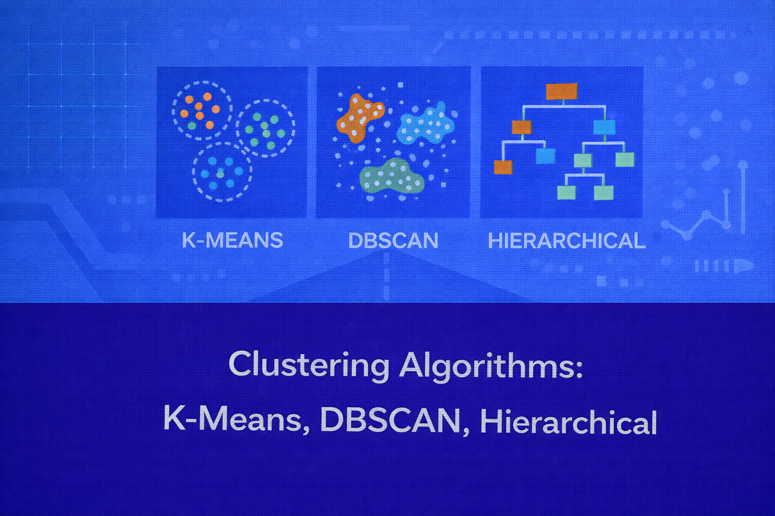
Clustering Algorithms: K-Means, DBSCAN, Hierarchical

Clustering is one of the most important families of unsupervised learning techniques. Its objective is to group unlabeled data points into meaningful subsets such that points within the same group are more similar to each other than to points in other groups. This whitepaper provides a deep technical explanation of three foundational clustering algorithms — K-Means, DBSCAN, and Hierarchical Clustering — with mathematical intuition, algorithmic details, evaluation criteria, computational trade-offs, interpretability considerations, and practical applications.

Abstract

Clustering is used when the target labels are unknown and the analyst wants to discover latent structure in data. Among many clustering methods, K-Means, DBSCAN, and Hierarchical Clustering are particularly influential because they represent three distinct philosophies: centroid-based partitioning, density-based grouping, and iterative agglomeration or division. This paper compares these approaches in detail, explains the underlying mathematics, discusses strengths and limitations, and shows when each method is most appropriate. All formulas are embedded inline in HTML-friendly format so the content can be pasted directly into WordPress or similar editors.

1. Introduction to Clustering

In supervised learning, the model learns from pairs (x, y), where x is an input and y is the known label. In clustering, the analyst only has observations X = {x1, x2, ..., xn}, where each xi ∈ ℝp, and the goal is to organize these points into groups without prior class assignments.

Informally, a “good” clustering has high intra-cluster similarity and low inter-cluster similarity. The exact meaning of similarity depends on the algorithm. In K-Means, similarity is typically expressed through Euclidean distance to a centroid. In DBSCAN, similarity is defined via neighborhood density. In Hierarchical Clustering, similarity is encoded through linkage criteria between points or groups.

2. Why Clustering Matters

Clustering is valuable because real-world data often contains hidden segments, regimes, or structures that are not explicitly labeled. Common use cases include customer segmentation, image grouping, anomaly screening, gene expression pattern discovery, document organization, geospatial hotspot discovery, network traffic profiling, and exploratory data analysis.

Unlike classification, clustering has no ground-truth labels during training. This makes the task both powerful and challenging: the analyst can discover new structure, but model evaluation becomes less direct and more dependent on assumptions or downstream usefulness.

3. General Clustering Framework

Let the dataset be X = {x1, ..., xn}. A clustering algorithm aims to produce either:

• a partition C = {C1, C2, ..., CK} of the dataset, or
• a hierarchy of nested clusters, or
• a set of dense regions plus noise points.

The right notion of a cluster depends on data geometry. Some datasets contain spherical, compact clusters. Others contain irregular shapes, chained structures, varying densities, or nested patterns. No single algorithm is best for all of these.

4. Distance and Similarity Measures

Many clustering algorithms require a measure of distance between points. The most common is Euclidean distance, d(x, z) = √[Σj=1p (xj - zj)2]. Other common choices include Manhattan distance, d(x, z) = Σj=1p |xj - zj|, Minkowski distance, cosine distance 1 - (xTz)/(||x|| ||z||), and Mahalanobis distance √[(x-z)TS-1(x-z)].

The choice of distance measure strongly affects the geometry of the resulting clusters. Feature scaling is also critical because distance-based methods can be dominated by variables with larger numerical ranges.

5. K-Means Clustering

K-Means is a centroid-based clustering algorithm that partitions the data into K non-overlapping clusters. Each cluster is represented by a centroid, usually the mean of the points assigned to that cluster.

5.1 Objective Function

K-Means seeks to minimize the within-cluster sum of squares, often called inertia or distortion. If μk is the centroid of cluster Ck, then the objective is:

Here, ||xi - μk||2 is the squared Euclidean distance between point xi and centroid μk. The algorithm attempts to find cluster assignments and centroids that minimize this objective.

5.2 Algorithmic Steps

Standard K-Means alternates between two steps:

• Assignment step: assign each point to its closest centroid, c(i) = argmink ||xi - μk||2.
• Update step: recompute each centroid as the mean of its assigned points, μk = (1 / |Ck|) Σxi ∈ Ck xi.

These steps are repeated until convergence, meaning assignments stop changing or the objective decreases by less than a tolerance threshold.

5.3 Why the Mean Appears

The centroid update is not arbitrary. For a fixed cluster assignment, the point minimizing Σ ||xi - μ||2 is the mean. This is why K-Means is specifically tied to squared Euclidean loss and compact, spherical cluster structure.

5.4 Initialization and K-Means++

K-Means is sensitive to initialization because the objective is non-convex and the algorithm can converge to local minima. Random initialization may lead to unstable results. K-Means++ improves initialization by choosing initial centroids with probability proportional to squared distance from existing centroids, which spreads them out and often improves convergence quality.

5.5 Computational Complexity

If n is the number of points, p the number of features, K the number of clusters, and T the number of iterations, then the rough cost of K-Means is O(n K p T). This makes it relatively efficient and scalable for large datasets, especially with optimized implementations or mini-batch variants.

5.6 Assumptions and Failure Modes

K-Means works best when clusters are compact, roughly spherical, and of similar size and density. It can perform poorly when clusters are elongated, overlapping, non-convex, or vary strongly in size. It is also sensitive to outliers because the mean shifts toward extreme points.

5.7 Interpretability

K-Means is interpretable because each cluster is summarized by a centroid. Analysts can examine centroid feature values to understand the “prototype” of each group. This makes K-Means popular in business segmentation tasks, where centroids can represent average customer profiles or average product usage patterns.

6. DBSCAN

DBSCAN stands for Density-Based Spatial Clustering of Applications with Noise. Unlike K-Means, it does not require the number of clusters to be specified in advance, and it can identify arbitrarily shaped clusters while explicitly labeling sparse points as noise.

6.1 Core Concepts

DBSCAN depends on two parameters: ε, the neighborhood radius, and MinPts, the minimum number of points needed to define a dense region.

The ε-neighborhood of a point xi is Nε(xi) = {xj : d(xi, xj) ≤ ε}.

A point is a core point if |Nε(xi)| ≥ MinPts. A point is a border point if it is not a core point but lies within the ε-neighborhood of a core point. A point is noise if it is neither core nor border.

6.2 Density Reachability and Connectivity

DBSCAN builds clusters using density reachability. A point xj is directly density-reachable from xi if xj ∈ Nε(xi) and xi is a core point.

A point is density-reachable from another if there exists a chain of direct density-reachability steps. Two points are density-connected if there exists some point from which both are density-reachable. DBSCAN defines clusters as maximal sets of density-connected points.

6.3 Algorithmic Logic

DBSCAN scans the dataset point by point. When it finds an unvisited core point, it starts a new cluster and expands that cluster by recursively or iteratively adding points that are density-reachable from it. Border points can be assigned to a cluster but do not themselves expand the cluster.

6.4 Advantages of DBSCAN

DBSCAN can discover non-spherical and arbitrarily shaped clusters. It is also robust to noise because isolated points remain unclustered. Unlike K-Means, it does not need a predefined K.

6.5 Limitations of DBSCAN

DBSCAN struggles when cluster densities differ substantially, because a single ε and MinPts may not fit all groups. It can also be sensitive to the choice of metric and parameter scale, especially in high-dimensional spaces where neighborhoods become less meaningful.

6.6 Choosing Parameters

A common heuristic is the k-distance plot. For each point, compute the distance to its k-th nearest neighbor, sort these distances, and look for an elbow. That elbow often suggests a reasonable ε. Typical choices for MinPts include values such as p + 1 or larger, depending on dimensionality and noise expectations.

6.7 Complexity

With a naive implementation, DBSCAN can require O(n2) distance checks. With spatial indexes such as KD-trees, Ball trees, or R-trees, practical performance can improve significantly, though gains diminish in high dimensions.

6.8 Interpretability

DBSCAN is interpretable in a geometric sense: clusters correspond to dense connected regions and noise corresponds to isolated points. This makes it especially useful in anomaly screening, geospatial analysis, and exploratory settings where outliers matter as much as cluster membership.

7. Hierarchical Clustering

Hierarchical Clustering builds a nested tree-like structure of clusters called a dendrogram. It comes in two main forms: agglomerative and divisive. Agglomerative clustering is much more common in practice.

7.1 Agglomerative Clustering

Agglomerative clustering starts with each point as its own cluster. At each step, it merges the two closest clusters. This process continues until all points are merged into a single cluster or until a desired number of clusters is reached.

7.2 Linkage Criteria

The notion of distance between clusters depends on the linkage rule:

• Single linkage: d(A, B) = minx ∈ A, z ∈ B d(x, z)
• Complete linkage: d(A, B) = maxx ∈ A, z ∈ B d(x, z)
• Average linkage: d(A, B) = (1 / (|A||B|)) Σx ∈ A Σz ∈ B d(x, z)
• Centroid linkage: d(A, B) = ||μA - μB||
• Ward’s method: merge the pair that yields the smallest increase in total within-cluster variance.

7.3 Ward’s Method

Ward linkage is especially important because it is closely related to K-Means. It merges the pair of clusters whose combination causes the smallest increase in Σ ||x - μ||2. This tends to produce compact, balanced clusters and is often preferred for numeric data with Euclidean structure.

7.4 Dendrogram Interpretation

A dendrogram visually represents the sequence of merges. The height at which two clusters are merged reflects the dissimilarity between them. By cutting the dendrogram at a chosen height, the analyst obtains a desired number of clusters. This makes Hierarchical Clustering particularly useful for exploratory analysis because it reveals multi-scale grouping structure rather than forcing a single partition immediately.

7.5 Divisive Clustering

Divisive clustering does the opposite: it starts with all data in one cluster and recursively splits clusters into smaller groups. While conceptually useful, divisive methods are generally more computationally demanding and less common in standard practice.

7.6 Complexity

Standard agglomerative clustering typically requires a pairwise distance matrix, which takes O(n2) memory and between O(n2 log n) and O(n3) time depending on implementation and linkage. This makes Hierarchical Clustering less scalable than K-Means for very large datasets.

7.7 Strengths and Limitations

Hierarchical Clustering does not require a prespecified number of clusters and offers strong interpretability through dendrograms. However, once a merge is made in agglomerative clustering, it cannot be undone, so early mistakes may propagate. Results are also sensitive to linkage choice and scaling.

8. Comparing the Three Algorithms

8.1 Clustering Philosophy

K-Means imposes a partition around centroids. DBSCAN grows dense regions and identifies noise. Hierarchical Clustering constructs a nested organization of the data. These are fundamentally different views of what a cluster is.

8.2 Number of Clusters

K-Means requires K in advance. DBSCAN infers the number of clusters from density structure. Hierarchical Clustering can be cut at different levels, so the number of clusters is chosen after the dendrogram is built.

8.3 Shape Sensitivity

K-Means favors convex and roughly spherical groups. DBSCAN is strong for arbitrary shapes such as rings, crescents, and density-connected manifolds. Hierarchical Clustering can capture a broader range of structures depending on linkage, though some linkages produce chaining effects or overly compact groupings.

8.4 Noise Handling

K-Means assigns every point to a cluster, even outliers. Hierarchical Clustering also tends to cluster all points unless preprocessing removes anomalies. DBSCAN is distinctive because it explicitly labels sparse points as noise.

8.5 Scalability

K-Means is generally the most scalable of the three, especially with mini-batch optimization. DBSCAN can scale reasonably with spatial indexing but depends on the data geometry. Hierarchical Clustering is usually the least scalable because of pairwise distance storage and repeated merges.

8.6 Interpretability

K-Means is interpretable through centroids and average cluster profiles. DBSCAN is interpretable through dense regions and noise labeling. Hierarchical Clustering is highly interpretable for exploratory work because the dendrogram exposes relationships at multiple granularities.

9. Cluster Evaluation

Since clustering is unsupervised, evaluation is less straightforward than in supervised learning. Several internal metrics are commonly used.

9.1 Silhouette Coefficient

For a point xi, let a(i) be the average distance to points in its own cluster, and b(i) the smallest average distance to points in any other cluster. The silhouette score is: s(i) = [b(i) - a(i)] / max(a(i), b(i)).

Values close to 1 suggest well-separated clustering, values near 0 suggest overlap, and negative values suggest possible misassignment.

9.2 Davies–Bouldin Index

This index measures average similarity between each cluster and its most similar other cluster. Lower values are better. It balances cluster scatter against centroid separation.

9.3 Calinski–Harabasz Index

This metric compares between-cluster dispersion to within-cluster dispersion. Higher values generally indicate better-defined clusters.

9.4 External Metrics

If ground truth labels are available for benchmarking, one may use Adjusted Rand Index, Normalized Mutual Information, homogeneity, completeness, or Fowlkes–Mallows. However, these are validation tools rather than assumptions available in genuine unsupervised discovery.

10. Feature Scaling and Preprocessing

For K-Means and most variants of Hierarchical Clustering, scaling is crucial because distance dominates the clustering behavior. Standardization using x'j = (xj - μj) / σj or min-max scaling using x'j = (xj - min(xj)) / (max(xj) - min(xj)) is often required.

Dimensionality reduction methods such as PCA are also commonly used before clustering to denoise data, reduce correlation, and improve geometric separation. In very high-dimensional spaces, raw Euclidean neighborhoods can become unstable.

11. Clustering in High Dimensions

High-dimensional data causes several issues. Distances concentrate, local neighborhoods become less meaningful, and the difference between “near” and “far” shrinks. This can harm K-Means and DBSCAN especially. Hierarchical methods also suffer because the pairwise distance matrix becomes less informative. In such cases, feature selection, dimensionality reduction, representation learning, or domain-specific similarity measures become essential.

12. Interpretability Advantages

Clustering often supports decision-making precisely because it compresses large unlabeled datasets into human-usable structures. K-Means offers centroid profiles that can be translated into segment personas. DBSCAN distinguishes structure from noise, which is useful in anomaly and hotspot analysis. Hierarchical Clustering offers an interpretable tree of relationships, making it easy to see which points or groups merge at what similarity level.

Interpretability, however, depends on thoughtful preprocessing, feature engineering, and domain context. A cluster can be mathematically coherent yet operationally meaningless if the wrong features or scales were used.

13. Practical Applications

13.1 Customer Segmentation

K-Means is often used to group customers based on behavior, spending, frequency, recency, and channel engagement. Centroids provide convenient summaries such as “high-value loyal customers” or “price-sensitive infrequent buyers.”

13.2 Geospatial Hotspot Discovery

DBSCAN is particularly strong in geospatial data because it can find dense geographic regions and separate isolated events as noise. This is useful in ride demand clustering, crime hotspot detection, logistics route analysis, and location intelligence.

13.3 Biological and Genomic Analysis

Hierarchical Clustering is widely used in gene expression studies because dendrograms reveal nested similarity among genes or samples. It is also useful when the analyst wants to explore relationships at multiple scales rather than commit to one fixed number of groups.

13.4 Document and Text Clustering

Documents represented through TF-IDF or embedding vectors can be clustered to organize corpora, discover topics, or support search exploration. K-Means is common in embedding spaces, while hierarchical methods are helpful when topic nesting is relevant.

13.5 Anomaly Screening

DBSCAN naturally supports anomaly identification because points not belonging to any dense region remain unlabeled as noise. This is often useful in sensor monitoring, cybersecurity, and transaction pattern analysis.

14. Choosing the Right Algorithm

K-Means is a strong choice when the analyst expects compact clusters, needs scalability, and wants interpretable centroids. DBSCAN is preferable when cluster count is unknown, shapes may be irregular, and noise handling is important. Hierarchical Clustering is most valuable when interpretability across multiple granularity levels matters and the dataset size is moderate enough to support pairwise structure.

In practice, algorithm choice should be driven by data geometry, scale, noise characteristics, interpretability needs, and the intended downstream action. There is rarely a universally best clustering algorithm.

15. Advantages and Limitations Summary

16. Best Practices

• Scale features before applying distance-based clustering.
• Use domain knowledge to choose meaningful variables.
• Visualize with PCA, t-SNE, or UMAP cautiously for exploration.
• Run multiple initializations for K-Means.
• Tune ε and MinPts carefully for DBSCAN.
• Experiment with linkage criteria in Hierarchical Clustering.
• Use internal validation metrics, but always verify business or scientific usefulness.

17. Conclusion

K-Means, DBSCAN, and Hierarchical Clustering each embody a different perspective on what it means for data to form a cluster. K-Means sees clusters as compact regions around centroids. DBSCAN sees them as dense connected components. Hierarchical Clustering sees them as nested relationships that unfold across scales. Understanding these conceptual differences is essential for choosing the right technique.

From a practical standpoint, clustering is not just a matter of running an algorithm. It requires careful decisions about feature representation, distance metrics, scaling, validation, and interpretability. When used thoughtfully, clustering can reveal powerful latent structure in unlabeled data and serve as a bridge between exploratory analysis and actionable segmentation.