Support Vector Machines (SVM)

Support Vector Machines are among the most elegant and mathematically grounded supervised learning algorithms. They are used for both classification and regression, and are especially valued for their geometric intuition, strong theoretical underpinnings, effectiveness in high-dimensional spaces, and the kernel trick that enables nonlinear decision boundaries without explicitly mapping data into higher dimensions.

1. Abstract

This whitepaper explains Support Vector Machines in depth, covering linear and nonlinear classification, the maximum-margin principle, support vectors, soft-margin optimization, dual formulations, kernel methods, multiclass extensions, and Support Vector Regression. The presentation is technical and detailed, with formulas embedded inline in HTML-friendly format suitable for WordPress or HTML editors.

2. Introduction

SVMs are supervised learning models that aim to find an optimal separating boundary between classes. Unlike many algorithms that simply try to minimize classification error on training data, SVMs optimize a stronger geometric criterion: they maximize the margin, the distance between the decision boundary and the nearest training points.

This idea gives SVMs several strengths:

• good generalization in many small- to medium-sized datasets
• robustness in high-dimensional feature spaces
• flexibility through kernel functions
• sparse solutions defined by support vectors
• strong theoretical basis through convex optimization

SVM was first introduced for binary classification, but the framework extends naturally to regression and multiclass learning.

3. Problem Setup

Assume a training set {(x_i, y_i)}_i=1ⁿ, where each feature vector x_i ∈ ℝ^d and each label for binary classification is y_i ∈ {-1, +1}. The goal is to learn a decision function that correctly predicts the class of unseen samples.

For a linear classifier, the decision function is f(x) = w^Tx + b, where w is the weight vector and b is the bias term. The prediction is given by ŷ = sign(w^Tx + b).

4. Linear SVM for Separable Data

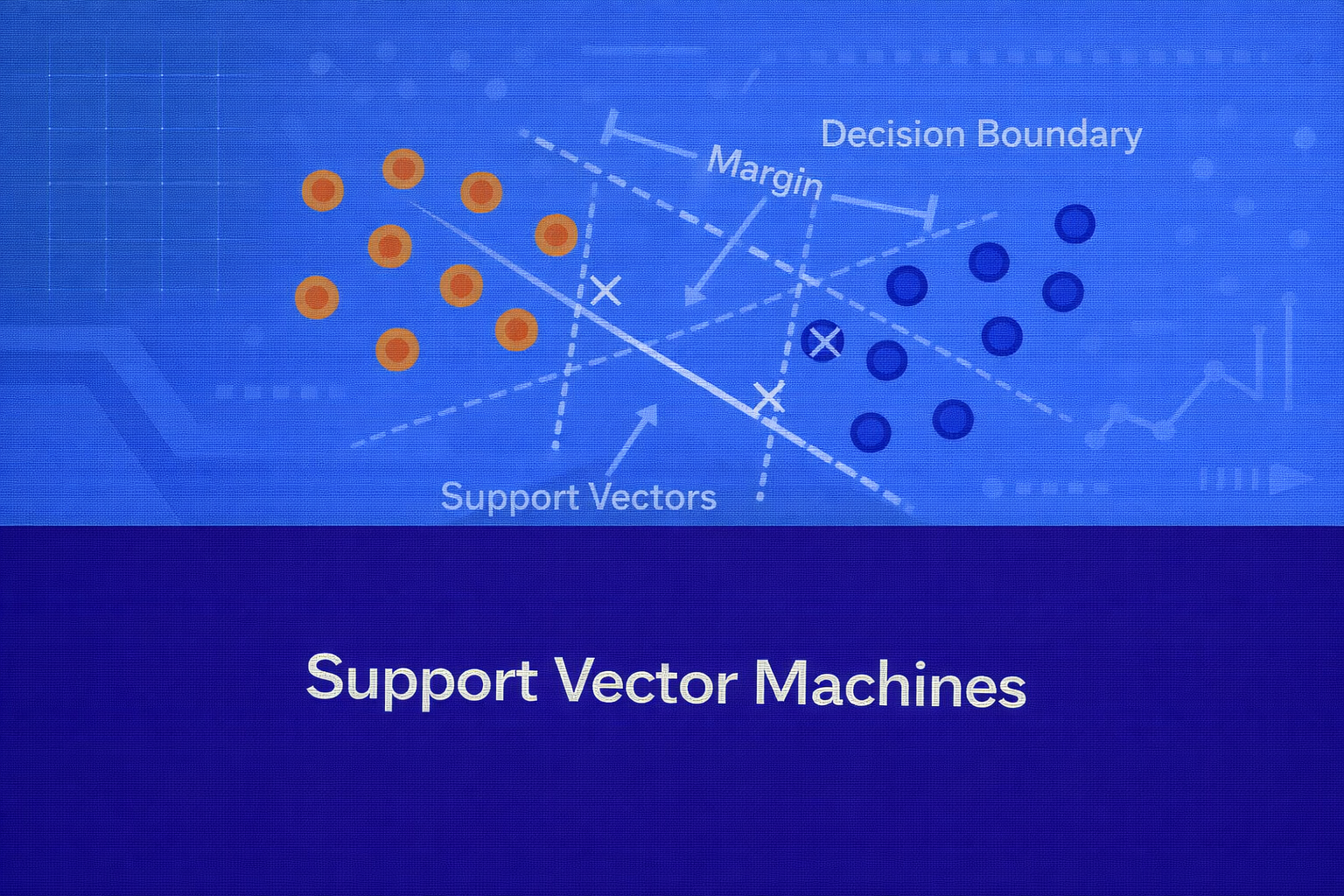
4.1 Separating Hyperplane

A hyperplane in d-dimensional space is defined by w^Tx + b = 0. A point is classified as positive if w^Tx + b > 0 and negative if w^Tx + b < 0.

For separable data, we require that every training point satisfies y_i(w^Tx_i + b) > 0. Since scaling w and b by the same positive constant does not change the hyperplane, SVM fixes the scale using the canonical constraints y_i(w^Tx_i + b) ≥ 1.

4.2 Margin

The geometric distance of a point x from the hyperplane is |w^Tx + b| / ||w||. For the closest points satisfying y_i(w^Tx_i + b) = 1, the distance to the boundary is 1 / ||w||. Therefore, the full margin between the two supporting hyperplanes w^Tx + b = 1 and w^Tx + b = -1 is 2 / ||w||.

Maximizing the margin is therefore equivalent to minimizing ||w||, or more conveniently (1/2)||w||².

4.3 Hard-Margin Optimization

The hard-margin SVM optimization problem is:

minimize over (w, b): (1/2) ||w||²

subject to: y_i(w^Tx_i + b) ≥ 1 for all i

This is a convex quadratic optimization problem with linear constraints, so it has a unique global optimum when the data is linearly separable.

5. Lagrangian and Dual Formulation

To solve the constrained optimization problem, we construct the Lagrangian:

L(w, b, α) = (1/2)||w||² – Σ_i=1ⁿ α_i[y_i(w^Tx_i + b) – 1]

where the Lagrange multipliers satisfy α_i ≥ 0.

The Karush-Kuhn-Tucker stationarity conditions give:

∂L/∂w = 0 ⇒ w = Σ_i=1ⁿ α_i y_i x_i

∂L/∂b = 0 ⇒ Σ_i=1ⁿ α_i y_i = 0

Substituting back yields the dual objective:

maximize over α: Σ_i=1ⁿ α_i – (1/2) Σ_i=1ⁿ Σ_j=1ⁿ α_i α_j y_i y_j x_i^Tx_j

subject to: α_i ≥ 0 and Σ_i=1ⁿ α_i y_i = 0

The optimal weight vector is then w = Σ α_i y_ix_i. Only points with α_i > 0 matter; these are the support vectors.

6. Role of Support Vectors

Support vectors are the training points lying closest to the decision boundary. They define the margin and fully determine the classifier. If a point is far from the boundary, its multiplier becomes zero and it does not influence the final solution.

This sparsity is one of the elegant properties of SVMs. The decision function becomes:

f(x) = Σ_{i ∈ SV} α_i y_i x_i^Tx + b

where SV denotes the set of support vectors.

7. Soft-Margin SVM

Real-world data is rarely perfectly separable. Hard-margin SVM fails when even a single violation exists. Soft-margin SVM introduces slack variables ξ_i ≥ 0 to allow margin violations and misclassifications.

The constraints become y_i(w^Tx_i + b) ≥ 1 – ξ_i, with ξ_i ≥ 0.

The optimization problem is:

minimize over (w, b, ξ): (1/2)||w||² + C Σ_i=1ⁿ ξ_i

subject to: y_i(w^Tx_i + b) ≥ 1 – ξ_i, ξ_i ≥ 0

The hyperparameter C controls the trade-off between margin maximization and training error minimization:

• large C penalizes violations heavily and prefers fewer classification errors
• small C allows more violations and prefers a wider margin

7.1 Hinge Loss View

Soft-margin SVM can be written using hinge loss. For each example, the hinge loss is max(0, 1 – y_i(w^Tx_i + b)). The unconstrained primal problem becomes:

minimize over (w, b): (1/2)||w||² + C Σ_i=1ⁿ max(0, 1 – y_i(w^Tx_i + b))

This makes the SVM connection to regularized empirical risk minimization explicit.

8. Nonlinear SVM and the Kernel Trick

Linear SVM works when classes are approximately separable by a hyperplane in the original feature space. But many real-world patterns are nonlinear. The core idea of kernel SVM is to map the input into a higher-dimensional feature space φ(x), then apply a linear SVM there.

Instead of computing φ(x) explicitly, SVM uses a kernel function K(x_i, x_j) = φ(x_i)^Tφ(x_j). This is the kernel trick.

The dual objective becomes:

maximize over α: Σ α_i – (1/2) Σ Σ α_i α_j y_i y_j K(x_i, x_j)

and the decision function becomes:

f(x) = Σ_{i ∈ SV} α_i y_i K(x_i, x) + b

This allows highly nonlinear boundaries while solving an optimization problem that depends only on pairwise similarities.

9. Common Kernel Functions

9.1 Linear Kernel

The linear kernel is K(x, z) = x^Tz. It produces the standard linear SVM and is often effective in high-dimensional sparse problems such as text classification.

9.2 Polynomial Kernel

The polynomial kernel is K(x, z) = (x^Tz + c)^d, where d is the degree and c is a constant. This implicitly models polynomial interactions between features.

9.3 Radial Basis Function (RBF) Kernel

The RBF or Gaussian kernel is K(x, z) = exp(-γ ||x – z||²). It is the most commonly used nonlinear kernel because it can model complex local structure.

The parameter γ controls the spread:

• small γ gives a smoother, broader influence
• large γ makes influence very local and may overfit

9.4 Sigmoid Kernel

The sigmoid kernel is K(x, z) = tanh(κ x^Tz + θ). It has historical connections to neural networks, though it is less commonly used in practice than linear or RBF kernels.

10. Choosing the Hyperparameters

For SVM, model performance depends heavily on hyperparameter selection:

• C: regularization strength
• γ: kernel width for RBF
• d: polynomial degree
• kernel type itself

Typical practice is cross-validation over a grid or logarithmic search space, for example C ∈ {10^-3, 10^-2, …, 10³} and γ ∈ {10^-3, 10^-2, …, 10²}.

11. Margin, Regularization, and Generalization

The margin is central to SVM generalization. A larger margin often implies lower model complexity and better robustness to unseen data. Soft-margin SVM combines this with empirical error control. This can be interpreted as minimizing a regularized objective (1/2)||w||² + C × loss, where the first term controls complexity and the second term controls fit to training data.

This gives SVM a clean bias-variance trade-off:

• very large C may produce low bias and high variance
• very small C may produce high bias and low variance

12. Geometric Interpretation

In linear classification, the decision boundary is the hyperplane w^Tx + b = 0. The two margin planes are w^Tx + b = +1 and w^Tx + b = -1. Support vectors lie on or within these boundaries in the soft-margin case.

In kernelized SVM, the data may be nonlinearly separable in original space but linearly separable in transformed feature space. The kernel lets us work with that transformed geometry implicitly.

13. Multiclass SVM

SVM is fundamentally a binary classifier, but multiclass problems are handled using decomposition strategies.

13.1 One-vs-Rest

Train one classifier per class. For class k, label all examples of class k as +1 and all others as -1. At inference, choose the class with the largest decision value.

13.2 One-vs-One

Train one classifier for each pair of classes. If there are K classes, the number of classifiers is K(K – 1)/2. Final prediction is made by voting or aggregation.

One-vs-one is commonly used in many SVM libraries because each binary problem is smaller and can be easier to optimize.

14. Support Vector Regression (SVR)

SVM also extends to regression through Support Vector Regression. Instead of trying to classify points, SVR tries to fit a function that deviates from the actual targets by no more than ε where possible, while remaining as flat as possible.

14.1 Linear SVR Objective

The SVR optimization problem introduces slack variables ξ_i and ξ_i^*:

minimize over (w, b, ξ, ξ^*): (1/2)||w||² + C Σ (ξ_i + ξ_i^*)

subject to: y_i – (w^Tx_i + b) ≤ ε + ξ_i

(w^Tx_i + b) – y_i ≤ ε + ξ_i^*

ξ_i, ξ_i^* ≥ 0

This creates an ε-insensitive tube around the regression function. Errors within ±ε are ignored; only larger deviations incur penalty.

14.2 ε-Insensitive Loss

The loss function for SVR is L_ε(y, f(x)) = max(0, |y – f(x)| – ε). This differs from squared error because it does not penalize small deviations inside the tube.

14.3 Kernel SVR

SVR also supports kernels. The resulting regression function becomes f(x) = Σ (α_i – α_i^*) K(x_i, x) + b. As in classification, only support vectors contribute to the final function.

15. Interpretability

Linear SVM is moderately interpretable because the coefficients in w show the orientation of the separating hyperplane. In text classification, for example, large positive or negative weights can indicate influential terms.

Kernel SVM is less interpretable because the model operates through support vectors and kernel similarities rather than explicit coefficients in the original input space. This reduces direct feature-level interpretability, though support vector inspection and local explanation methods can still help.

16. Advantages of SVM

• strong performance in high-dimensional spaces
• effective when number of features exceeds number of samples
• convex optimization yields global optimum
• kernel trick allows flexible nonlinear modeling
• sparse solution through support vectors
• works well on text, bioinformatics, image subproblems, and medium-sized tabular datasets

17. Limitations of SVM

• training can become expensive on very large datasets
• kernel methods scale poorly with large n because of the kernel matrix
• hyperparameter tuning is crucial and sometimes delicate
• kernel SVM is less interpretable than linear models or trees
• probabilities are not native and often require calibration such as Platt scaling
• sensitive to feature scaling, especially with RBF kernels

18. Feature Scaling and Preprocessing

SVM is highly sensitive to the relative scale of features because dot products and distances directly affect the optimization and kernel computation. Standardization is usually essential, especially for RBF or polynomial kernels.

A common transformation is x’_j = (x_j – μ_j) / σ_j, where μ_j is the mean and σ_j is the standard deviation of feature j.

19. Evaluation Metrics

For classification, SVM is typically evaluated with accuracy, precision, recall, F1-score, ROC-AUC, and confusion matrices depending on the class distribution and business objective.

For regression, SVR is evaluated with metrics such as MSE = (1/n) Σ (y_i – ŷ_i)², RMSE = sqrt(MSE), MAE = (1/n) Σ |y_i – ŷ_i|, and R² = 1 – RSS/TSS.

20. Practical Model Selection Guidance

Linear SVM is a strong choice when the dataset is high-dimensional and approximately linearly separable, particularly in sparse domains like text. Kernel SVM, especially with RBF, is often useful when relationships are nonlinear and the dataset is not too large. SVR is attractive when you want a robust regression method with an ε-insensitive loss and potentially nonlinear function fitting through kernels.

In practice:

• start with a linear kernel as a baseline
• scale features before training
• use cross-validation for C, γ, and ε
• monitor overfitting when γ is large or C is extreme
• use calibrated probabilities if downstream business logic needs probabilities rather than margins

21. SVM vs Logistic Regression

Both linear SVM and logistic regression learn linear decision boundaries, but they optimize different objectives. Logistic regression minimizes log loss and models probabilities directly using P(y=1|x) = 1 / (1 + e^-(wTx+b)). SVM minimizes hinge loss and focuses on maximizing margin.

Linear SVM objective can be written as (1/2)||w||² + C Σ max(0, 1 – y_if(x_i)), while logistic regression uses Σ log(1 + e^-y_if(x_i)) up to scaling and regularization. Logistic regression is usually preferred when calibrated probabilities matter; SVM is often preferred when margin-based separation and high-dimensional robustness are priorities.

22. SVM vs Decision Trees and Ensembles

SVM tends to work well with dense geometry and smooth class boundaries, especially after feature scaling. Tree-based models handle mixed feature types, missing-value strategies, non-monotonic interactions, and tabular heterogeneity more naturally. Kernel SVM can outperform trees in structured medium-sized classification settings, but trees and ensembles often scale better operationally and are easier to explain at a decision-rule level.

23. Conclusion

Support Vector Machines remain one of the most important classical machine learning methods because they combine geometry, optimization, and statistical learning theory in a highly elegant way. The central idea is simple but powerful: find the boundary with the largest margin. Soft margins make the model practical, dual optimization makes the sparse support-vector representation possible, and kernels make nonlinear learning computationally feasible without explicitly engineering high-dimensional features.

For classification, SVM offers robust margin-based learning. For regression, SVR offers flexible function estimation through the ε-insensitive framework. While deep learning and ensemble methods dominate many modern workflows, SVM remains a critical tool for practitioners who need strong performance, mathematical rigor, and reliable behavior in high-dimensional or medium-sized datasets.