Decision Trees and Random Forests are foundational tree-based learning methods used for both prediction and classification on structured data. They are especially valued because they can model nonlinear relationships, automatically capture interactions, work with mixed feature types, and offer a stronger interpretability story than many black-box methods. This whitepaper explains their mathematical formulation, splitting logic, ensemble mechanics, optimization intuition, evaluation, and interpretability advantages, with formulas embedded inline in HTML-friendly form so the content can be pasted into WordPress.
1. Introduction
Tree-based models do not assume a global linear relationship between inputs and outputs. Instead, they partition the feature space into smaller regions and attach a prediction rule to each region. A Decision Tree learns a sequence of hierarchical rules such as “if feature x_j < s, go left; otherwise, go right.” This recursive partitioning is expressive enough to represent threshold effects, nonlinear dependencies, and interaction effects without manual feature crossing.
However, single Decision Trees are unstable. Small changes in data can produce a substantially different tree. Random Forests solve this by averaging many decorrelated trees. The result is usually much better generalization while preserving much of the structural intuition of trees.
2. Problem Setup
Assume a supervised learning dataset D = {(x_i, y_i)}i=1n, where each input vector is x_i = [x_{i1}, x_{i2}, …, x_{ip}]T. For classification, the target is categorical, typically y_i ∈ {1, 2, …, K}. For regression, the target is continuous, meaning y_i ∈ ℝ. The model seeks to learn a function f(x) that minimizes out-of-sample prediction error.
3. Decision Trees
3.1 Core Idea
A Decision Tree recursively partitions the input space into disjoint regions R_1, R_2, …, R_M, then predicts a constant value or class within each region. Formally, the tree can be written as f(x) = Σm=1M c_m I(x ∈ R_m), where c_m is the output assigned to region R_m and I(·) is the indicator function.
For classification, c_m is usually the majority class or a class-probability vector. For regression, c_m is usually the mean target value of the training observations falling into that leaf.
3.2 Recursive Binary Splitting
At a given node, the algorithm examines candidate splits over all features and thresholds. For feature j and threshold s, the split creates two child regions: R_{left}(j,s) = {x | x_j < s} and R_{right}(j,s) = {x | x_j ≥ s}. The best split is the one that produces the largest impurity reduction.
This process is greedy: each split is selected to optimize local gain at the current node, not the globally optimal entire tree. That makes training tractable, but it also means the learned tree is not guaranteed to be globally optimal.
3.3 Classification Trees and Node Impurity
Suppose node t contains N_t samples. Let the class proportion for class k inside that node be p(k|t) = (1/N_t) Σ I(y_i = k, x_i ∈ t). A pure node contains only one class; an impure node contains a mix of classes.
Three common impurity measures are used.
Misclassification error is E(t) = 1 – max_k p(k|t). This is intuitive but often too coarse for split selection because it changes only when the dominant class changes.
Gini impurity is G(t) = 1 – Σk=1K p(k|t)2. Gini is widely used in CART-style trees because it is smooth, computationally efficient, and sensitive to class mixing.
Entropy is H(t) = – Σk=1K p(k|t) log p(k|t). Entropy comes from information theory and measures uncertainty in the class distribution.
For a split from parent node t into children t_L and t_R, impurity after the split is the weighted average (N_{t_L}/N_t) I(t_L) + (N_{t_R}/N_t) I(t_R). Information gain is therefore IG = I(t) – [(N_{t_L}/N_t) I(t_L) + (N_{t_R}/N_t) I(t_R)]. The chosen split maximizes IG or equivalently minimizes the weighted child impurity.
3.4 Regression Trees and Squared Error
For regression, impurity is usually based on squared error. If node t contains response values y_i, then the optimal constant prediction for that node is the sample mean c_t = (1/N_t) Σ y_i. The node error is SSE(t) = Σ (y_i – c_t)2. For any candidate split, the algorithm minimizes the post-split objective SSE(t_L) + SSE(t_R).
This makes regression trees piecewise-constant estimators. They can fit nonlinear surfaces, but their outputs are step-like rather than smooth.
3.5 Tree Construction Procedure
A typical Decision Tree is built as follows. Start with all training data in the root. Enumerate candidate splits over features and thresholds. Select the split with best impurity reduction. Create left and right child nodes. Repeat recursively on each child until a stopping rule is triggered.
Common stopping rules include maximum depth, minimum samples required to split, minimum samples per leaf, zero impurity, or minimum gain threshold. These are crucial because unrestricted growth typically leads to overfitting.
3.6 Prediction
Prediction is simple: traverse the tree from the root to a terminal node using the learned decision rules. For classification, the output is often argmax_k p(k|leaf). For regression, it is usually the leaf mean.
3.7 Bias-Variance Behavior
Single trees usually have low bias but high variance. They are flexible and can fit complex patterns, but because they are sensitive to small data perturbations, their predictions can vary considerably across training samples. This instability is the major reason ensembles like Random Forests are so effective.
3.8 Overfitting and Pruning
A fully grown tree can memorize noise and idiosyncratic local patterns. To prevent this, one may use pre-pruning or post-pruning. Pre-pruning limits growth using constraints such as depth or minimum leaf size. Post-pruning grows a larger tree first and then removes branches that do not justify their complexity.
In cost-complexity pruning, one minimizes C_α(T) = Σm=1|T| N_m Q_m(T) + α|T|, where |T| is the number of terminal nodes, Q_m(T) is the leaf impurity or error, and α penalizes larger trees. Larger α values encourage smaller, simpler trees.
3.9 Interpretability Advantages of Decision Trees
Decision Trees are strongly interpretable because each prediction corresponds to a decision path. A path can be rendered as a rule, for example: if age ≥ 35 and income < 50000 and prior_default = 0, then predict approval. This rule-based structure is intuitive for domain experts and decision-makers.
The model is also interpretable globally because the overall structure can often be visualized. Features near the root typically have broad influence, and splits deeper in the tree refine specialized subpopulations. This is much easier to explain than neural network activations or dense latent representations.
3.10 Strengths of Decision Trees
Decision Trees naturally capture nonlinear effects and feature interactions, require little preprocessing, do not require feature scaling, and support both classification and regression. They work well when the domain itself is rule-like, with policy thresholds or segmented behavior.
3.11 Weaknesses of Decision Trees
Their main weaknesses are instability, overfitting tendency, and limited predictive power compared with strong ensembles. Deep trees can also become hard to interpret because local branches proliferate. In regression, their piecewise-constant predictions can be too coarse when a smooth response surface is needed.
4. Random Forests
4.1 Why Random Forests Were Introduced
Random Forests were introduced to reduce the high variance of Decision Trees without dramatically increasing bias. They combine two key ideas: bootstrap aggregation, also called bagging, and random feature subsampling. Together these mechanisms produce many different trees whose errors are less correlated, and averaging them yields better generalization.
4.2 Bagging
Bagging trains multiple models on bootstrap samples. A bootstrap sample is obtained by sampling n training instances with replacement from the original dataset of size n. Because sampling is with replacement, some observations appear multiple times while others are omitted. Each tree is trained on its own bootstrap dataset.
If the b-th tree is denoted f_b(x), then for regression the bagged prediction is f_{bag}(x) = (1/B) Σb=1B f_b(x). For classification, the ensemble predicts by majority vote, written as ŷ = mode{f_1(x), f_2(x), …, f_B(x)}.
Averaging reduces variance because fluctuations that are idiosyncratic to individual trees partially cancel out.
4.3 Random Feature Subsampling
Bagging alone still allows strong predictors to dominate all trees, causing correlation across the ensemble. Random Forests address this by considering only a random subset of features at each split. If the total number of features is p, only m features are considered when searching for the best split, where typically m < p. Common defaults are m ≈ sqrt(p) for classification and m ≈ p/3 for regression.
This forced randomness means different trees explore different predictive structures, reducing correlation and improving the benefit of averaging.
4.4 Random Forest Algorithm
For b = 1, 2, …, B, draw a bootstrap sample from the training set. Grow a tree on that sample. At each node, sample m candidate features from the full set of p features. Choose the best split only from those m features. Grow the tree fully or near-fully, often without pruning. After all B trees are trained, aggregate their predictions by averaging or voting.
4.5 Out-of-Bag Estimation
Each bootstrap sample omits about one-third of the training observations on average. These omitted observations are called out-of-bag, or OOB, samples for that tree. Because each training point is OOB for many trees, Random Forests can estimate generalization performance without a separate validation set.
If B_i is the set of trees for which observation i was OOB, then its OOB prediction is obtained by aggregating only those trees: f_{OOB}(x_i) = (1/|B_i|) Σb∈B_i f_b(x_i) for regression, or majority vote for classification. Aggregating these OOB predictions across the training set gives an almost-free internal estimate of test error.
4.6 Why Random Forests Reduce Variance
Suppose each tree has variance σ2 and pairwise correlation ρ. The variance of the average of B such trees is approximately ρσ2 + ((1-ρ)/B)σ2. This shows two important points. First, increasing B reduces the second term. Second, decreasing correlation ρ is critical. Random Forests therefore rely not only on averaging many trees, but on making those trees different enough to matter.
4.7 Classification and Regression in Random Forests
For classification, each tree outputs a class label or class-probability estimate, and the forest aggregates these to produce the final class. For regression, each tree outputs a number, and the final prediction is the arithmetic average. This averaging makes Random Forest regression much smoother and more stable than a single regression tree.
4.8 Hyperparameters
The most important Random Forest hyperparameters are the number of trees B, the number of features considered at each split m, maximum depth, minimum samples per split, minimum samples per leaf, and whether class balancing or sample weighting is used. Increasing B usually improves stability until performance plateaus, while increasing depth increases variance and local fit.
4.9 Feature Importance
Random Forests provide useful feature importance measures. One common approach is mean decrease in impurity, which sums the impurity reductions attributable to each feature across all trees. Another is permutation importance, which measures the drop in model performance when a feature’s values are randomly permuted. Permutation importance is often more reliable because it reflects effect on predictive performance rather than just split frequency.
4.10 Interpretability Advantages of Random Forests
Random Forests are less directly interpretable than a single tree because the model consists of many trees rather than one rule set. Even so, they are often more interpretable than many other high-performing methods because practitioners can inspect feature importance, partial dependence, individual conditional expectation patterns, proximity structures, OOB behavior, and representative trees.
In practice, the interpretability advantage is relative. A single tree gives strong local and global transparency. A Random Forest sacrifices some direct transparency in exchange for much better predictive reliability, while still preserving a meaningful explanation toolkit.
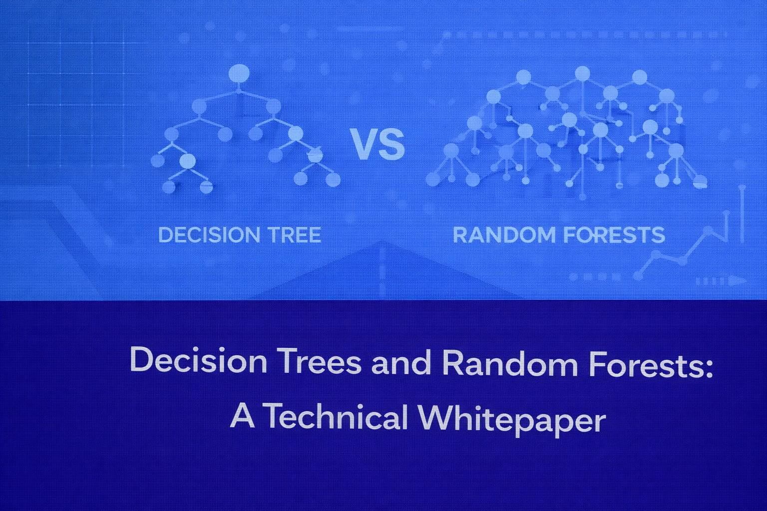
5. Decision Trees vs Random Forests
A Decision Tree is a single hierarchical rule model. It is easy to explain end to end, but it has high variance and often lower predictive accuracy. A Random Forest is an ensemble of many trees trained on randomized views of the data. It is usually far more accurate and stable, but less directly explainable than one tree.
Decision Trees are preferable when exact rule extraction, transparency, and policy articulation dominate. Random Forests are preferable when predictive performance, robustness, and automatic interaction learning are more important than having one compact decision structure.
6. Mathematical View of Tree Predictions
Both Decision Trees and Random Forests can be viewed as adaptive partitioning estimators. A tree defines regions of the input space and assigns a constant to each region. A forest averages many such adaptive partitions. This is why forests can model highly nonlinear decision surfaces even though each individual tree uses only simple threshold splits.
For classification, the forest can be interpreted probabilistically as estimating P(y=k|x) through average leaf-level class proportions across trees. For regression, it estimates the conditional expectation E[y|x] by averaging leaf means from multiple randomized trees.
7. Evaluation Metrics
For classification, Decision Trees and Random Forests are commonly evaluated with accuracy (TP + TN)/(TP + TN + FP + FN), precision TP/(TP + FP), recall TP/(TP + FN), F1-score 2(PR)/(P+R), ROC-AUC, and PR-AUC. For regression, common metrics are mean squared error MSE = (1/n) Σ (y_i – ŷ_i)2, root mean squared error, and mean absolute error MAE = (1/n) Σ |y_i – ŷ_i|.
Random Forests often outperform single trees on these metrics because they reduce overfitting while preserving nonlinear flexibility.
8. Practical Considerations
Trees require little preprocessing. Feature scaling is usually unnecessary because splits depend on order, not magnitude. Missing-value handling depends on the implementation; some libraries support surrogate splits or built-in handling, while others require imputation. Trees can also handle mixed numeric and encoded categorical inputs reasonably well.
Random Forests are computationally heavier than single trees because many trees must be trained, but they parallelize very well. In high-dimensional tabular data, they are often an excellent baseline and frequently a competitive final model.
9. Limitations
Single trees are unstable and easily overfit. Random Forests reduce that variance but are still not perfect. They can become memory-intensive, may be slower at inference than a single tree, and their feature importance can be biased in some settings, particularly with high-cardinality features or strongly correlated variables. They also do not extrapolate smoothly in regression beyond the range of training responses.
10. When to Use Which
Use a Decision Tree when interpretability is the dominant requirement, when you need explicit rules, or when the decision process itself must be communicated and audited. Use a Random Forest when you want a strong, low-maintenance, nonlinear baseline for structured data, especially when predictive stability matters more than having one compact decision path.
11. Conclusion
Decision Trees and Random Forests occupy a crucial place in machine learning because they bridge interpretability and predictive capability. A Decision Tree offers transparent, human-readable rule extraction and naturally aligns with decision-making workflows. A Random Forest extends that idea into a more powerful ensemble by combining many randomized trees, reducing variance and improving robustness. Together they illustrate an important theme in machine learning: a simple, interpretable base learner can often be transformed into a much stronger predictive system through ensemble design.
For practitioners, the key is not to treat these models as merely beginner methods. Understanding impurity, recursive partitioning, pruning, bagging, feature subsampling, OOB estimation, and importance analysis provides a deep foundation for tree-based learning in both classical and modern machine learning pipelines.