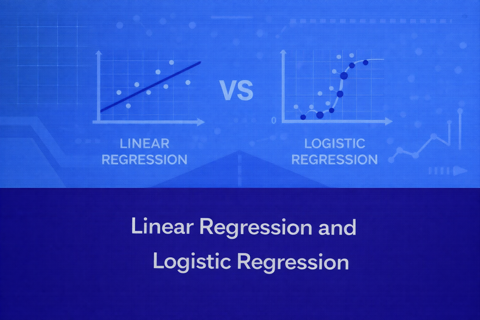
Linear Regression and Logistic Regression

1. Introduction

Regression models are among the earliest and most interpretable forms of predictive modeling. Their continued relevance comes from strong statistical grounding, computational efficiency, interpretability, applicability to baseline modeling, ease of deployment, and compatibility with feature engineering and regularization.

Despite the rise of deep learning and ensemble methods, Linear Regression and Logistic Regression remain indispensable because they help practitioners answer not only what to predict, but also why predictions arise.

At a high level:

• Linear Regression models the expected value of a continuous response as a linear combination of input features.
• Logistic Regression models the probability of class membership using a nonlinear transformation of a linear combination of input features.

Their shared structure makes them conceptually related, but their loss functions, output interpretations, and statistical assumptions differ significantly.

2. Problem Formulation

Let the dataset contain n observations and p predictor variables.

Let the feature vector for the i-th sample be:

Let the target be:

• yi ∈ ℝ for Linear Regression
• yi ∈ {0,1} for binary Logistic Regression

Let the parameter vector be:

where β0 is the intercept. The generic linear predictor is:

or in compact form:

3. Linear Regression

3.1 Objective

Linear Regression predicts a continuous target value by fitting a linear relationship between the input variables and the output.

The predicted value is:

The residual for observation i is:

3.2 Matrix Formulation

Prediction becomes:

3.3 Estimation by Ordinary Least Squares

The most common estimation method is Ordinary Least Squares (OLS), which minimizes the Residual Sum of Squares (RSS):

Substituting the model:

In matrix notation:

To minimize this, differentiate with respect to β and set to zero:

This yields the normal equations:

Assuming XTX is invertible, the OLS solution is:

3.4 Statistical Assumptions of Linear Regression

3.4.1 Linearity

3.4.2 Independence of Errors

3.4.3 Homoscedasticity

3.4.4 Normality of Errors

3.5 Interpretation of Coefficients

Holding all other variables constant, a one-unit increase in xj changes the expected value of y by β̂j units.

3.6 Variance of the Estimator

3.7 Hypothesis Testing in Linear Regression

3.8 Goodness of Fit

3.9 Optimization Perspective

3.10 Diagnostics and Failure Modes

Residual plots help detect nonlinearity, heteroscedasticity, omitted variable effects, and outliers. Multicollinearity is commonly assessed through the Variance Inflation Factor (VIF):

3.11 Regularized Linear Regression

Ridge Regression

Lasso Regression

Elastic Net

3.12 When Linear Regression Works Well

Linear Regression is suitable when the target is continuous, the relationship is approximately linear in parameters, interpretability is important, and a strong baseline model is needed quickly.

3.13 Limitations of Linear Regression

• poor fit for highly nonlinear relationships unless engineered features are introduced
• sensitive to outliers
• assumes constant variance under classical inference
• cannot naturally bound outputs
• unsuitable for classification tasks

4. Logistic Regression

4.1 Objective

Logistic Regression is a probabilistic classification model. It is used when the response variable is categorical, particularly binary classification.

4.2 Why Not Use Linear Regression for Classification?

For classification, this is problematic because predictions are unbounded, error variance is not constant, probability relationships are nonlinear, and thresholding linear outputs is statistically suboptimal.

4.3 Logistic Function

4.4 Log-Odds Interpretation

This is called the logit link. Logistic Regression is linear in the log-odds, not directly in the probability.

4.5 Interpretation of Coefficients

A one-unit increase in xj changes the log-odds by βj, holding other variables constant. Equivalently, it multiplies the odds by eβj.

4.6 Likelihood Formulation

4.7 Maximum Likelihood Estimation

4.8 Gradient and Optimization

Common optimization methods include batch gradient descent, stochastic gradient descent, mini-batch gradient descent, Newton-Raphson, Iteratively Reweighted Least Squares (IRLS), and L-BFGS.

Newton-Raphson Update

4.9 Decision Rule

Otherwise predict class 0. In cost-sensitive or imbalanced settings, a different threshold may be better than 0.5.

4.10 Assumptions of Logistic Regression

Logistic Regression assumes correct functional form in the log-odds, independence of observations, no perfect multicollinearity, adequate sample size, and absence of complete separation.

4.11 Evaluation Metrics for Logistic Regression

4.12 Regularized Logistic Regression

4.13 Extensions of Logistic Regression

This is the softmax form used in multinomial Logistic Regression.

4.14 When Logistic Regression Works Well

Logistic Regression is highly effective when the classification boundary is approximately linear in transformed feature space, interpretability matters, and probabilistic output is required.

4.15 Limitations of Logistic Regression

• linear decision boundary in feature space unless features are engineered
• may underperform on highly nonlinear patterns
• sensitive to extreme multicollinearity
• can struggle under complete or quasi-complete separation
• threshold choice matters
• class imbalance can distort naive accuracy interpretation

5. Linear Regression vs Logistic Regression

Linear Regression predicts a continuous number. Logistic Regression predicts a probability, which is then converted to a class label.

Linear Regression uses squared error loss and typically OLS estimation. Logistic Regression uses log loss and maximum likelihood estimation. Linear Regression coefficients describe changes in expected output; Logistic Regression coefficients describe changes in log-odds or odds ratios.

For Logistic Regression, this is the decision boundary when the classification threshold is 0.5 because:

6. Geometric Perspective

OLS projects the target vector y onto the column space of X. The fitted values ŷ are the orthogonal projection of y onto that subspace. Residuals are orthogonal to the column space:

Logistic Regression learns a linear separator in feature space, but scores are converted into probabilities through the sigmoid. The boundary is a hyperplane:

7. Bias-Variance Considerations

Both models face the bias-variance trade-off. High bias can result from under-engineered features, omitted interactions, or too much regularization. High variance can result from too many features, noisy data, multicollinearity, weak regularization, or overfitting small datasets.

8. Feature Engineering Considerations

Both Linear and Logistic Regression are sensitive to representation quality. Useful transformations include polynomial terms, interaction terms, log transforms, binning, standardization, and one-hot encoding.

This remains linear in parameters even though it is nonlinear in x.

9. Numerical and Implementation Details

Feature scaling improves numerical stability and gradient-based convergence. Categorical features should be one-hot encoded with care to avoid the dummy variable trap. Missing values must be imputed, modeled explicitly, or removed. Outliers affect Linear Regression strongly due to squared loss and can also distort Logistic Regression through high leverage in feature space.

10. Practical Diagnostics Checklist

10.1 For Linear Regression

• residual vs fitted plots
• Q-Q plots for residual normality
• heteroscedasticity tests
• VIF for multicollinearity
• leverage and Cook’s distance
• train-test performance gap

10.2 For Logistic Regression

• confusion matrix at chosen threshold
• ROC-AUC and PR-AUC
• calibration
• multicollinearity
• class imbalance
• separation issues
• coefficient stability across folds

11. Calibration and Probability Quality

Logistic Regression often provides well-calibrated probabilities, especially compared to some more complex models. This makes it highly useful in medical decision support, finance risk scoring, insurance underwriting, and policy-driven threshold systems.

12. Computational Complexity

Linear Regression solved via matrix inversion can become expensive for large feature spaces because of operations involving:

Logistic Regression requires iterative optimization, so its computational cost depends on solver choice, number of iterations, number of features, and data sparsity.

13. Common Misconceptions

• Logistic Regression is not “regression” in the same operational sense as Linear Regression; it is primarily a classification model.
• Linear Regression should not generally be used for classification by thresholding outputs.
• A linear model can still capture nonlinear relationships through transformed features while remaining linear in parameters.
• Logistic Regression outputs probabilities first; class labels are obtained by thresholding.
• High accuracy alone does not imply a good classification model, especially in imbalanced data.

14. Use Cases by Business Context

14.1 Linear Regression

Best suited for revenue prediction, demand forecasting, property valuation, time-to-resolution estimation, energy consumption estimation, and pricing optimization.

14.2 Logistic Regression

Best suited for customer churn classification, loan default prediction, fraud detection screening, lead conversion prediction, disease diagnosis support, and click/no-click modeling.

15. Summary Table in Narrative Form

Linear Regression predicts numeric outcomes using a linear combination of input features and is typically estimated by minimizing squared error. Logistic Regression predicts class probabilities by applying a sigmoid transformation to a linear score and is estimated by maximizing likelihood or minimizing log loss. Linear Regression assumes a continuous dependent variable and is evaluated using RMSE, MAE, and R². Logistic Regression assumes binary or categorical outcomes and is evaluated using accuracy, precision, recall, F1-score, ROC-AUC, PR-AUC, and log loss. Coefficients in Linear Regression are interpreted as changes in the expected output, while coefficients in Logistic Regression are interpreted as changes in log-odds or odds ratios.

16. Conclusion

Linear Regression and Logistic Regression remain cornerstone models because they combine statistical rigor, interpretability, and practical usability. Linear Regression provides a principled way to model continuous outcomes and estimate marginal effects under explicit assumptions. Logistic Regression extends the linear modeling paradigm into classification by modeling probabilities through the logistic link, preserving interpretability while aligning the model with binary outcome behavior.

From a machine learning standpoint, both models are not merely simple baselines. They are often the correct production choice when the data generating process is sufficiently structured, when transparency matters, when compliance or auditability is needed, or when a robust first model is required before exploring more complex alternatives.

A mature practitioner should understand not only how to fit these models, but also how to diagnose them, regularize them, interpret them, and recognize when their assumptions break.